


For low temperature thermometry, negative temperature coefficient (NTC) temperature sensors such as germanium, Cernox™, and ruthenium oxide (Rox™) can provide tremendous sensitivity and resolution. While the resistance as a function of temperature characteristic is somewhat fixed for a given model of Rox temperature sensors, it can vary greatly for germanium RTDs where fabrication is accomplished through bulk doping during crystal growth and for Cernox™ where fabrication is accomplished through thin film deposition. For both germanium and Cernox™ RTDs there is a common misconception that a higher resistance equates to a better sensor. This is a somewhat ambiguous statement, but for the purposes of this discussion, “better sensor” is interpreted as better resolution or better accuracy (i.e., lower uncertainty). This application note addresses the question “Is higher resistance better?” for NTC temperature sensors.
Instrumentation
It is important to understand that concepts of resolution and accuracy are largely meaningless if applied only to the temperature sensor. These concepts become meaningful only when discussed in the framework of the electronics that are used to measure their resistance. While the physical construction of the sensor may limit the allowable excitation power to avoid or minimise self-heating, it is ultimately the electronic resolution and electronic accuracy of the instrument that determines the temperature resolution and temperature accuracy of the overall measurement. Even then, the electronic resolution and accuracy will depend upon the resistance range and excitation power level.
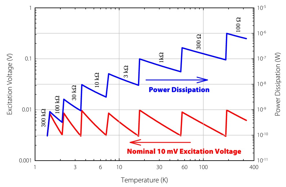
As temperature decreases below 20 K, the thermal conductivity of the materials used to construct temperature sensors decreases rapidly, thus limiting the thermal connection of the sensor to its environment. This requires that the power dissipated in the sensor be decreased as temperature is decreased to avoid self-heating the sensor. For NTC temperature sensors it is common to operate them at “constant voltage” over large portions of their temperature range. Since the resistance increases as temperature decreases, the power dissipated in the sensor decreases with temperature as required for an NTC device operated in this manner. For a germanium, Cernox™, or Rox™ RTD, a nominal 10 mV excitation voltage works well over the temperature range spanning 1.4 K to room temperature. In reality, however, the voltage is not constant. Virtually all cryogenic temperature controllers and monitors operate as constant current sources. Even when the excitation is set in terms of voltage, the instrument provides a constant current related to VSet/RRange. On a given resistance range, this means that the true excitation voltage signal, VExc, varies from 0 V to VSet and it equals VSet only at full scale on that resistance range. Obviously, when the resistance drops too low for one resistance range, the instrument should switch to the next lower resistance range. This requires an increase in current to keep the ratio VSet/RRange nearly constant. The overall result is an excitation voltage signal that is sawtooth-shaped with drops occurring where the resistance range changes occur.
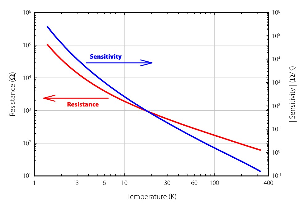
As an example, consider a model CX-1050 with resistance and sensitivity as a function of temperature shown in Figure 1. The measurement instrument is a Lake Shore Model 340 temperature controller with a nominal excitation of 10 mV from 1.4 K to 325 K. Specifications for this controller are in the Lake Shore product catalogue or at www.lakeshore.com . The Model 340 temperature controller resistance ranges have upper limits of 30 Ω, 100 Ω, 300 Ω, 1kΩ, 3 kΩ, 10 kΩ, 30 kΩ, 100 kΩ and 300 kΩ, and it is assumed that the CX-1050 temperature sensor is measured on the lowest resistance range that can be used. Then the excitation current, IExc, is given by VSet/RRange where VSet=10 mV. The actual excitation voltage is given by VExc = IExc,× RMeas where RMeas is the measured temperature dependent resistance of the sensor. Figure 2 shows the actual voltage excitation and power dissipation as a function of temperature for the sample CX-1050-SD. Notice that as the resistance range changes the voltage excitation and power dissipation abruptly change resulting in the saw tooth shape of each curve. The resistance range for each segment of the two curves is labelled. The nominal 10 mV excitation is achieved only at full scale on a given resistance range.
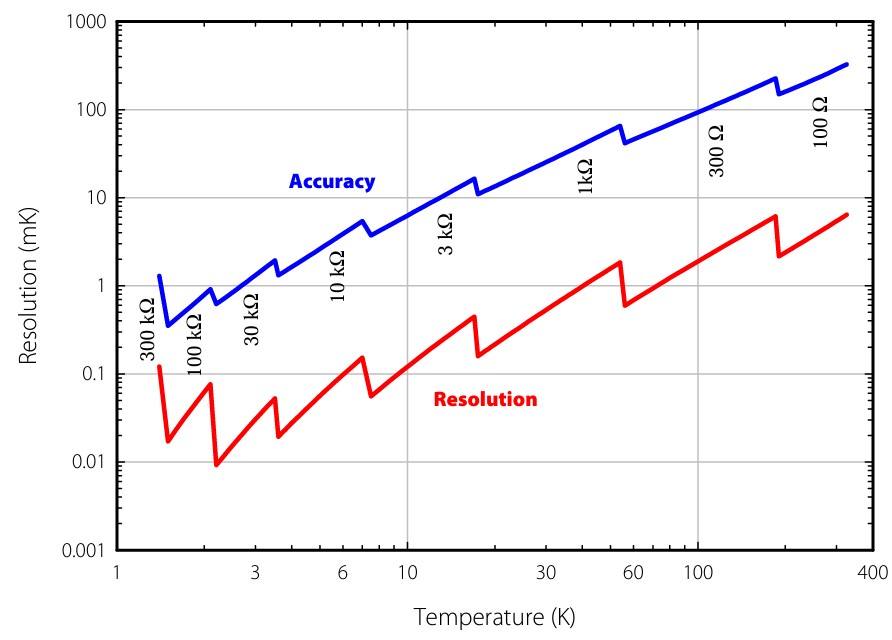
Just as the power dissipation depends upon the set excitation level and resistance range, so do both the resolution and accuracy (uncertainty) of the measurement as shown in Figure 3. Again, the resistance range for each segment of the two curves is listed. Also notice that while the sensitivity of the CX-1050 continues to increase rapidly at the lowest temperatures, the best temperature resolution occurs around 3.5 K on the 30 kΩ scale, demonstrating that the measurement can become more difficult to perform when the resistance is too high or too low.
Another complication is that as the sensor resistance changes due to changing temperature, it may be undesirable to change from 100% range on one scale to 30% range on the next adjacent scale (or vice versa, depending on whether temperature is increasing or decreasing.) In the best case, this could simply result in an annoying or unanticipated change in power dissipation, resolution, and accuracy. In the worst case, this could create an unstable control temperature if the resistance at the control temperature lies at the boundary of two ranges, causing the controller to constantly switch ranges while controlling at that temperature. To avoid this, most instruments are purposely designed to have some overlap between ranges. The downside is that in automatic mode the instrument may switch resistance ranges at different percentages of full range, depending upon whether resistance is increasing or decreasing. In these cases, the only way to truly know the resistance range and consequently the power dissipation, resolution and accuracy is to query the instrument.
Sensor Resistance
With an understanding of the instrumentation, the question remains as to whether higher resistance with its associated higher sensitivity implies better resolution and accuracy for an NTC temperature sensor. Resistances that are too high (greater than a few hundred kilohms) or too low (less than 10 ohms) are more difficult to measure than resistances that lie between the two extremes. Instrument specifications can degrade as either extreme is approached. This portion of the discussion will examine the resolution and accuracy for low, moderate, and high resistance sample Cernox™ sensors. The labelling refers to the resistance at the lowest temperature for which each Cernox™ model is designed to be useful (0.1 K for CX-1010 and 1.4 K for CX-1030). Low, moderate, and high resistance is somewhat arbitrary and is a trade-off between being high enough to give reasonable resolution, but not too high as to be difficult to measure. For the remainder of this discussion low resistance refers to 5 kΩ, moderate resistance refers to 50 kΩ, and high resistance refers to 100 kΩ. The actual resistance and sensitivity values for each sensor used in this analysis are plotted in Figures 4 and 5.
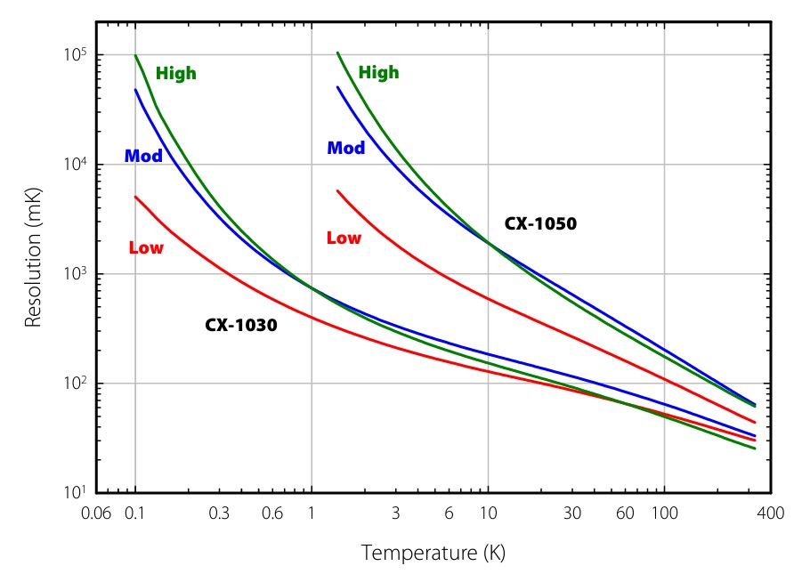
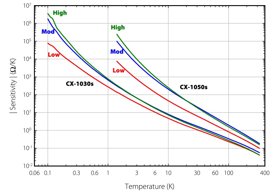
As pointed out before, the concepts of resolution and accuracy are meaningless without the details of the instrumentation used to perform the measurement. In these two examples, the CX-1010 is measured using a Lake Shore Model 370 AC resistance bridge while the CX-1050 is measured using a Lake Shore Model 340 temperature controller.
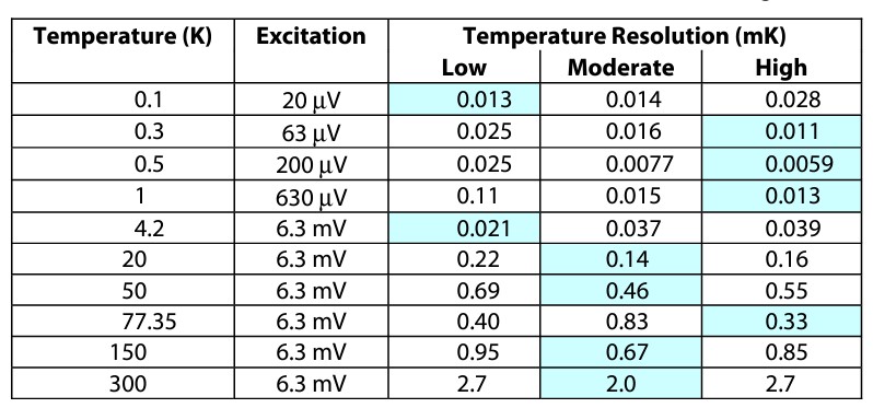
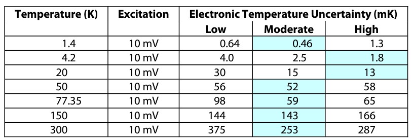
Specifications for both are available in the Lake Shore product catalogue or at www.qd-uki.co.uk. Based upon each individual sensor’s response curve and the instrument specifications, the temperature resolution and accuracy was computed for each sample. The results are given in Tables 1 and 2 for the CX-1010 measured using the Lake Shore Model 370 and in Tables 3 and 4 for the CX-1050 measured using the Lake Shore Model 340. The best values are back-shaded in each table to help guide the eye. Note that the electronic temperature uncertainty listed in Tables 2 and 4 do not include calibration uncertainty.

As seen in Tables 1 and 2 for CX-1010s measured using a Lake Shore Model 370 AC resistance bridge, the best resolution varies among all three resistance ranges with the upper resistance ranges being slightly better while the best temperature uncertainty is split between the moderate and high resistance ranges with the high resistance range being slightly better. The same is mostly true for the CX-1050s measured with a Lake Shore Model 340 shown in Tables 3 and 4.
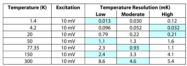
In this case, the moderate resistance range gives the best temperature uncertainty. In addition, at a particular temperature, the resistance range that gives the best resolution does not even necessarily give the best accuracy. The main reason for the variation in the best sensor is that the higher sensor resistance forces the instrument to a higher resistance range, and the electronic resistance and accuracy at higher ranges can degrade faster than the sensitivity increases. Three points can be made here. First, the higher sensitivity does not necessarily translate into higher temperature resolution. In fact, in both of these examples, the low resistance samples have a sensitivity 100 times less than the high resistance samples at their lowest operating temperature, yet the low resistance samples give better resolution. Second, the high resistance samples do not necessarily provide the best temperature measurement uncertainty. There is a trend, but it is not absolute. Third, even though the relative sensitivities can differ significantly (two orders of magnitude at the lower temperatures) the differences in resolution and sensitivity are mostly within a factor of 2 among the three resistance ranges at any given temperature.
It could be argued that the results from Tables 1 through 4 are skewed by virtue of operating at “constant” voltage. In this mode, a low resistance sensor would dissipate more power (P=V2/R) than a higher resistance sensor. Since using a higher power to measure the resistance usually yields better specifications, this may make the low resistance sensors look better than they are. In fact, this is not the case. Normalising the measurement power to the moderate resistance sample for all three samples in the group yields results that are reasonably consistent with the results in Tables 1 through 4.
Conclusions
There are many instrumentation subtleties that affect low temperature thermometry measurements, including the excitation mode and how the instrument switches between resistance ranges. Ultimately the excitation level and resistance range determine the electronic resolution and accuracy, which in turn determine the temperature resolution and accuracy. Since for a given NTC thermometer type higher resistance implies higher sensitivities, it would be expected that the higher resistance thermometers should yield better resolution and accuracy. As demonstrated, this is not the case in general. The “best” sensor in terms of temperature resolution and accuracy is somewhat random in that it depends on which resistance range the instrument is forced to operate. Overall, the low resistance samples perform as well as the high resistance samples and the differences that do occur are generally less than a factor of two.

The Lake Shore Cryotronics range is sold exclusively in the UK and Ireland through Quantum Design UK and Ireland.
For more information, please contact our Technical Sales Engineer, Dr. Alex Murphy by email or call (01372) 378822.


